Then the run time difference between solver routine 1A and 1B becomes clear.
| Top-left cell = MIN 1st row = supply 1st column = demand All other cells = transport cost per quantity |
In this case, demand should be met by supply against minimal transportation costs. The table below shows demand, supply and the transportation cost per quantity for each supply-demand connection. Note that total demand equals total supply (no requirement as such). With r referring to row, and c to column, and Xrc to the transport quantity from Supplyr to Demandc, and Crc to the transport cost per quantity from Supplyr to Demandc the LP problem can be formulated as:
Minimize Σ Crc × Xrc , subject to
Σ Xrc ≥ Demandc ∀ c
Σ Xrc ≤ Supplyr ∀ r
Xrc ≥ 0 ∀ r,c
Minimize Σ Crc × Xrc , subject to
Σ Xrc ≥ Demandc ∀ c
c
Σ Xrc ≤ Supplyr ∀ r
r
Xrc ≥ 0 ∀ r,c
Demo data
| COST PER QUANTITY | SUPPLY | ||||||||||
| 14 | 15 | 16 | 18 | 9 | 4 | 7 | 15 | 20 | 232 | ||
| DEMAND | 40 | 334 | 356 | 336 | 18 | 45 | 795 | 59 | 291 | 89 | 585 |
| 14 | 285 | 234 | 805 | 283 | 440 | 325 | 957 | 330 | 796 | 600 | |
| 26 | 431 | 965 | 600 | 241 | 190 | 417 | 117 | 916 | 631 | 436 | |
| 18 | 763 | 719 | 550 | 396 | 200 | 619 | 689 | 514 | 108 | 874 | |
| 10 | 484 | 933 | 792 | 607 | 322 | 548 | 851 | 715 | 802 | 272 | |
| 30 | 816 | 611 | 225 | 79 | 851 | 425 | 841 | 481 | 500 | 903 | |
| 18 | 899 | 391 | 165 | 155 | 657 | 231 | 757 | 730 | 48 | 282 | |
| 8 | 922 | 320 | 661 | 38 | 726 | 760 | 150 | 891 | 483 | 407 | |
| 4 | 316 | 504 | 123 | 587 | 938 | 706 | 382 | 729 | 547 | 310 | |
| 6 | 751 | 37 | 825 | 754 | 140 | 323 | 229 | 592 | 571 | 914 | |
| 6 | 117 | 706 | 414 | 674 | 275 | 703 | 395 | 315 | 115 | 891 | |
| 12 | 498 | 898 | 858 | 498 | 187 | 411 | 717 | 353 | 560 | 368 | |
| 18 | 169 | 470 | 643 | 433 | 132 | 652 | 898 | 719 | 555 | 444 | |
| 2 | 840 | 336 | 860 | 577 | 112 | 292 | 422 | 294 | 411 | 474 | |
| 20 | 935 | 569 | 443 | 639 | 523 | 549 | 60 | 415 | 409 | 791 | |
| 32 | 753 | 614 | 610 | 426 | 136 | 578 | 118 | 335 | 751 | 494 | |
| 20 | 83 | 572 | 108 | 570 | 241 | 946 | 651 | 762 | 790 | 40 | |
| 36 | 167 | 838 | 963 | 299 | 362 | 90 | 843 | 39 | 50 | 45 | |
| 28 | 517 | 657 | 914 | 79 | 678 | 811 | 173 | 364 | 930 | 593 | |
| 2 | 746 | 440 | 747 | 392 | 946 | 456 | 560 | 462 | 798 | 462 | |
Optimal quantities: total costs are 102587
| OPTIMAL QUANTITIES | SUPPLY | ||||||||||
| 14 | 15 | 16 | 18 | 9 | 4 | 7 | 15 | 20 | 232 | ||
| DEMAND | 40 | 4 | 9 | 2 | 2 | 23 | |||||
| 14 | 1 | 9 | 4 | ||||||||
| 26 | 26 | ||||||||||
| 18 | 18 | ||||||||||
| 10 | 10 | ||||||||||
| 30 | 16 | 14 | |||||||||
| 18 | 18 | ||||||||||
| 8 | 8 | ||||||||||
| 4 | 4 | ||||||||||
| 6 | 6 | ||||||||||
| 6 | 6 | ||||||||||
| 12 | 12 | ||||||||||
| 18 | 7 | 11 | |||||||||
| 2 | 2 | ||||||||||
| 20 | 7 | 13 | |||||||||
| 32 | 32 | ||||||||||
| 20 | 20 | ||||||||||
| 36 | 36 | ||||||||||
| 28 | 28 | ||||||||||
| 2 | 2 | ||||||||||
Add network problem specifics to the solution
Enter data tab separated (copy-paste from Excel file) or semicolon separated.Nodes
NodeID | Supply_Min* | Supply_Max* | Costs_In | Costs_Out | Throughput_Min | Throughput_Max
* Supply >0 = supply node, <0 = demand node, 0 = balanced througput node
Arcs
ArcID | From_NodeID | To_NodeID | Costs | Flow_Min | Flow_MaxIntro
You can define a netwok consisting of nodes and arcs. The decision variables in this type of problem are the arc quantities. Each arc has a cost per quantity (e.g. transportation costs), a lowerbound (minimum flow quantity) and upperbound (maximum flow quantity). Each node has supply quantity (demand = negative supply).Demo case
The graph below shows a minimum cost flow problem. The arcs are labeled with pairs of numbers: the first number is the capacity and the second number is the cost. The number in parentheses next to a node represent supply or demand. Node 0 is a supply node that supplies 20, while nodes 3 and 4 are demand nodes (or: sink nodes) that demand 5 and 15 respectively (demand = negative supply).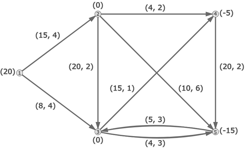
Advanced node modeling options
For modeling convenience this web app offers advanced node modeling options:- Each node has a cost per incoming and outgoing quantity (e.g. inbound and outbound warehouse handling costs).
- Each node has flexible supply/demand (supply upper and lowerbound), so - for example - a node may supply between 0 and 1000, or have a demand between 6 and 10 (entered as a negative supply between -10 and -6). If demand/supply is not flexible, then enter the same value for both Min and Max.
- Each node has a throughput upper and lowerbound. Throughput could be either based on incoming or outgoing quantity. We have (arbitrarily) chosen incoming quantity as the basis.
General network modeling remarks
- By adding dummy nodes and arcs you can create completely balanced systems, and make a model 'better readible'.
- Other network flow software may not offer advanced node modeling options.
- You can create node upper and lowerbounds by splitting a node in two nodes, adding a zero costs arc in between, and setting upper and lowerbound at this arc (connecting all original incoming arcs to the first node, all original outgoing arcs to the second).
- You can create a node with flexible demand/supply by adding a dummy node that 'eats' any non-used over-supply at zero costs (creating a balanced system in which total supply equals total demand).
- Incoming/outgoing node costs can be transferred/added to all incoming/outgoing arcs of the node.
- A network model can be used to model transitions in time, with an arc representing a transition from time to time+1.
Enter data tab separated (copy-paste from Excel file) or semicolon separated.
The tableau is prefilled with the transportation problem demo case. Putting the demo case table next to this Simplex tableau you will recognize the numbers. Note that instead of Xrc (20 rows × 10 columns) all has been translated into Xj (200 variables sitting on a single row), so Xr=6,c=3 has become X53 that has a value of 16 in the optimal solution. If you run "Solve network minimum cost flow problem" the tableau is filled with the translation of the network flow problem demo case.
| LP problem input = Simplex tableau. The format is explained below the text area. |
Standard LP problem formulation
Maximize ΣCi × Xi , subject to Σ (Aij × Xi) ≤ Bj ∀ j , and Xi ≥ 0 ∀ i
You can also minimize and/or use ≥ and = as restriction type as shown by the demo cases. See also: wikipedia: Linear Programmingi
i
Simplex tableau legend
- Top row contains the cost factors.
- 1st cell = MIN (minimize) or MAX (maximize). MIN is default in logistics. Though the standard LP problem formulation is about maximizing profit (MAX), logistics problems are usually about minimizing costs (MIN).
- 2nd cell = initial goal value = always 0.
- 3rd and next cells = costs factors Ci. Each of these column 'belongs to' one decision variable (X_1, X_2,...).
- All other rows formulate the constraints.
- 1st cell = constraint type <= or >= or =
- 2nd cell = constraint value Bj
- 3rd and next cells = values of Aij (optional: can be left empty if zero). Each of these columns 'belongs to' one decision variable (X_1, X_2,...)
Normally you need to setup - so called - slack variables as well (read: dummy variables required for the Simplex method to work).
Do not enter slack variables! They are created automatically.
Do not enter slack variables! They are created automatically.
The tableau is prefilled with the transportation problem demo case. Putting the demo case table next to this Simplex tableau you will recognize the numbers. Note that instead of Xrc (20 rows × 10 columns) all has been translated into Xj (200 variables sitting on a single row), so Xr=6,c=3 has become X53 that has a value of 16 in the optimal solution. If you run "Solve network minimum cost flow problem" the tableau is filled with the translation of the network flow problem demo case.
The solution will appear here, once run.