Excel Bilinear and spline based interpolation functions within 2‑dimensional table

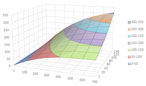
Visualisation of the data table above

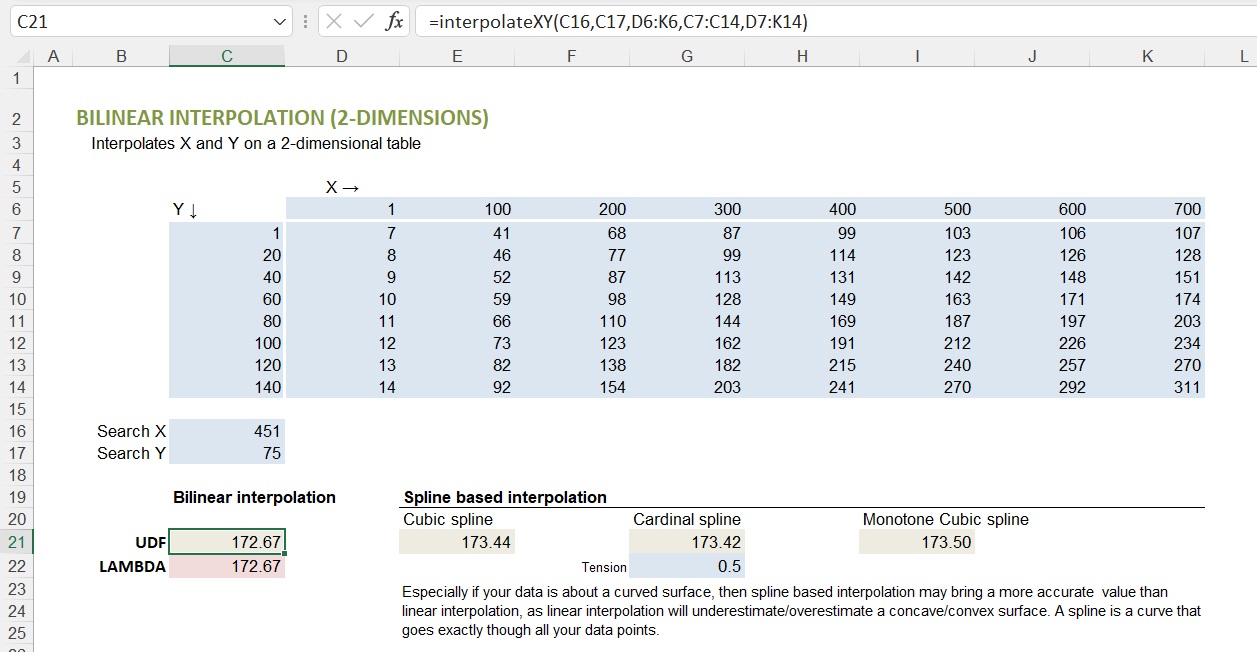
Calculation
X = 451 lies between X = 400 and X = 500. X-fraction = (451 - 400)/(500 - 400) = 0.51
Y = 75 lies between Y = 60 and Y = 80. Y-fraction = (75 - 60)/(80 - 60) = 0.75

The 4 data point values to interpolate between are (X,Y):
     1. (400,60) = 149
     2. (500,60) = 163
     3. (400,80) = 169
     4. (500,80) = 187

Interpolation X:
     1.&2. → 149 + 0.51 × (163 - 149) = 156.14
     3.&4. → 169 + 0.51 × (187 - 169) = 178.18

Interpolation Y:
     156.14 + 0.75 × (178.18 - 156.14) = 172.67 = final bilineair interpolation result.

The Cubic spline based interpolation brings 173.44, which is 0.4% higher. If your data is about a concave curved surface, it is obvious that the bilinear interpolation result will always slightly underestimate, except on a data point itself. The above example is slightly convex in Y direction, but more dominantly concave in X direction.

Bilinear interpolation - VBA code to be put in a module

In MS Excel, press Alt+F11 to open the Visual Basic Editor (Windows). Via top menu: Insert → Module. Copy the code below into the module.

User Defined Function (UDF)Public Function InterpolateXY(ByRef X As Range, ByRef Y As Range, ByRef XRange As Range, ByRef YRange As Range, ByRef ValueTable As Range) As Double 'if X or Y fall outside the table, the function result is an error value If (X < WorksheetFunction.Min(XRange)) Or (X > WorksheetFunction.Max(XRange)) Or (Y < WorksheetFunction.Min(YRange)) Or (Y > WorksheetFunction.Max(YRange)) Then InterpolateXY = CVErr(xlErrNA) Exit Function End If Dim X1, X2, Y1, Y2, PX1, PX2, PY1, PY2, V1, V2, V3, V4, FX, FY, C12, C34 'Determine data table points around searchvalues X1 = WorksheetFunction.XLookup(X, XRange, XRange, , -1) X2 = WorksheetFunction.XLookup(X, XRange, XRange, , 1) Y1 = WorksheetFunction.XLookup(Y, YRange, YRange, , -1) Y2 = WorksheetFunction.XLookup(Y, YRange, YRange, , 1) PX1 = WorksheetFunction.Match(X1, XRange, 0) PX2 = WorksheetFunction.Match(X2, XRange, 0) PY1 = WorksheetFunction.Match(Y1, YRange, 0) PY2 = WorksheetFunction.Match(Y2, YRange, 0) V1 = ValueTable(PY1, PX1) V2 = ValueTable(PY1, PX2) V3 = ValueTable(PY2, PX1) V4 = ValueTable(PY2, PX2) 'X and Y fractions If (X2 = X1) Then FX = 0 Else FX = (X - X1) / (X2 - X1) If (Y2 = Y1) Then FY = 0 Else FY = (Y - Y1) / (Y2 - Y1) '2 intermediate results after interpolation on X C12 = V1 + FX * (V2 - V1) C34 = V3 + FX * (V4 - V3) 'final result after interpolation on Y InterpolateXY = C12 + FY * (C34 - C12) End Function

LAMBDA function L_InterpolateXY

Dependent on your Excel setting you need to use semicolon or comma in formulas. Best is to open the demo file and copy the formula from there, as it will contain your local settings. Else - if required - copy in function in text editor and replace comma by semicolon before copying into Excel.

Based on L_InterpolateX, so you need to copy in both functions.

Lambda function XY=LAMBDA(searchx,searchy,rangeX,rangeY,valuerange,LET(valuerange,INDEX(valuerange,1,0),L_InterpolateX(searchx,rangeX,OFFSET(valuerange,MATCH(XLOOKUP(searchy,rangeY,rangeY,,-1),rangeY,0)-1,0))+IF(XLOOKUP(searchy,rangeY,rangeY,,-1)=searchy,0,(searchy-XLOOKUP(searchy,rangeY,rangeY,,-1))/(XLOOKUP(searchy,rangeY,rangeY,,1)-XLOOKUP(searchy,rangeY,rangeY,,-1))*(L_InterpolateX(searchx,rangeX,OFFSET(valuerange,MATCH(XLOOKUP(searchy,rangeY,rangeY,,1),rangeY,0)-1,0))-L_InterpolateX(searchx,rangeX,OFFSET(valuerange,MATCH(XLOOKUP(searchy,rangeY,rangeY,,-1),rangeY,0)-1,0))))))

LAMBDA function L_InterpolateX

Lambda function X=LAMBDA(searchvalue,searchrange,valuerange, LET(LB,XLOOKUP(searchvalue,searchrange,searchrange,,-1),UB,XLOOKUP(searchvalue,searchrange,searchrange,,1),LV,XLOOKUP(searchvalue,searchrange,valuerange,,-1),UV,XLOOKUP(searchvalue,searchrange,valuerange,,1), IF(OR(searchvalue<MIN(searchrange),searchvalue>MAX(searchrange)),NA(),LV+IF(LB=searchvalue,0,(searchvalue-LB)/(UB-LB)*(UV-LV)))))

Spline based 2-D interpolation - Main functions and sub functions VBA code

VBA code Public Function interpolateXY_CubicSpline(ByRef x As Range, ByRef y As Range, ByRef XRange As Range, ByRef YRange As Range, ByRef ValueTable As Range) As Double 'if X or Y fall outside the table, the function result is an error value If (x < WorksheetFunction.Min(XRange)) Or (x > WorksheetFunction.Max(XRange)) Or (y < WorksheetFunction.Min(YRange)) Or (y > WorksheetFunction.Max(YRange)) Then interpolateXY_CubicSpline = CVErr(xlErrNA) Exit Function End If Dim X1, X2, Y1, Y2, PX1, PX2, PY1, PY2, V1, V2, V3, V4, FX, FY, C12, C34 Dim i As Long i = YRange.Count Dim arr() As Double ReDim arr(i) For i = 0 To YRange.Count - 1 'transpose as assumption is input in regular table format arr(i) = CubicSpline_SP(WorksheetFunction.Transpose(XRange), WorksheetFunction.Transpose(ValueTable.Rows(i + 1)), x) Next interpolateXY_CubicSpline = CubicSpline_SP(YRange, WorksheetFunction.Transpose(arr), y) End Function Public Function interpolateXY_CardinalSpline(ByRef x As Range, ByRef y As Range, ByRef XRange As Range, ByRef YRange As Range, ByRef ValueTable As Range, tension As Single) As Double 'if X or Y fall outside the table, the function result is an error value If (x < WorksheetFunction.Min(XRange)) Or (x > WorksheetFunction.Max(XRange)) Or (y < WorksheetFunction.Min(YRange)) Or (y > WorksheetFunction.Max(YRange)) Then interpolateXY_CardinalSpline = CVErr(xlErrNA) Exit Function End If Dim X1, X2, Y1, Y2, PX1, PX2, PY1, PY2, V1, V2, V3, V4, FX, FY, C12, C34 Dim i As Long i = YRange.Count Dim arr() As Double ReDim arr(i) For i = 0 To YRange.Count - 1 'transpose as assumption is input in regular table format arr(i) = CardinalSpline_SP(WorksheetFunction.Transpose(XRange), WorksheetFunction.Transpose(ValueTable.Rows(i + 1)), tension, x) Next interpolateXY_CardinalSpline = CardinalSpline_SP(YRange, WorksheetFunction.Transpose(arr), tension, y) End Function Public Function interpolateXY_MonotoneCubicSpline(ByRef x As Range, ByRef y As Range, ByRef XRange As Range, ByRef YRange As Range, ByRef ValueTable As Range) As Double 'if X or Y fall outside the table, the function result is an error value If (x < WorksheetFunction.Min(XRange)) Or (x > WorksheetFunction.Max(XRange)) Or (y < WorksheetFunction.Min(YRange)) Or (y > WorksheetFunction.Max(YRange)) Then interpolateXY_MonotoneCubicSpline = CVErr(xlErrNA) Exit Function End If Dim X1, X2, Y1, Y2, PX1, PX2, PY1, PY2, V1, V2, V3, V4, FX, FY, C12, C34 Dim i As Long i = YRange.Count Dim arr() As Double ReDim arr(i) For i = 0 To YRange.Count - 1 'transpose as assumption is input in regular table format arr(i) = MonotoneCubicSpline_SP(WorksheetFunction.Transpose(XRange), WorksheetFunction.Transpose(ValueTable.Rows(i + 1)), x) Next interpolateXY_MonotoneCubicSpline = MonotoneCubicSpline_SP(YRange, WorksheetFunction.Transpose(arr), y) End Function Public Function CubicSpline_SP(DatapointsX, DatapointsY, ByVal atX As Single) As Double Dim n, i As Long Dim xin, yin As Variant Dim p, sig, h, b, a, k As Double Dim klo, khi As Long Dim X1, X2 'trick: transpose to get rid of second dimension of range - with input data sitting in a regular table with records in rows xin = Application.Transpose(DatapointsX) yin = Application.Transpose(DatapointsY) n = UBound(xin) ReDim u(n - 1) As Single ReDim yt(n) As Single yt(1) = 0 u(1) = 0 For i = 2 To n - 1 sig = (xin(i) - xin(i - 1)) / (xin(i + 1) - xin(i - 1)) p = sig * yt(i - 1) + 2 yt(i) = (sig - 1) / p u(i) = (yin(i + 1) - yin(i)) / (xin(i + 1) - xin(i)) - (yin(i) - yin(i - 1)) / (xin(i) - xin(i - 1)) u(i) = (6 * u(i) / (xin(i + 1) - xin(i - 1)) - sig * u(i - 1)) / p Next i yt(n) = 0 For i = n - 1 To 1 Step -1 yt(i) = yt(i) * yt(i + 1) + u(i) Next i X1 = WorksheetFunction.XLookup(atX, xin, xin, , -1) X2 = WorksheetFunction.XLookup(atX, xin, xin, , 1) klo = WorksheetFunction.Match(X1, xin, 0) khi = WorksheetFunction.Match(X2, xin, 0) If (klo = khi) Then CubicSpline_SP = yin(klo) Else h = xin(khi) - xin(klo) a = (xin(khi) - atX) / h b = (atX - xin(klo)) / h CubicSpline_SP = a * yin(klo) + b * yin(khi) + ((a ^ 3 - a) * yt(klo) + (b ^ 3 - b) * yt(khi)) * (h ^ 2) / 6 End If End Function Public Function CardinalSpline_SP(DatapointsX, DatapointsY, ByVal tension As Single, atX) Dim xin As Variant, yin As Variant Dim ptsX() Dim ptsY() Dim iRow, i, op, r As Long Dim n As Integer Dim t, thi, tlo, x, xnow, y As Double Dim klo, khi As Long Dim X1, X2 'trick: transpose to get rid of second dimension of range xin = Application.Transpose(DatapointsX) yin = Application.Transpose(DatapointsY) n = UBound(xin) 'sort in ascending X order Dim tmp If xin(1) > xin(n) Then 'swap values For i = 1 To WorksheetFunction.RoundDown(n / 2, 0) tmp = xin(i) xin(i) = xin(n + 1 - i) xin(n + 1 - i) = tmp tmp = yin(i) yin(i) = yin(n + 1 - i) yin(n + 1 - i) = tmp Next End If ReDim ptsX(n + 2) ReDim ptsY(n + 2) For i = 1 To n ptsX(i) = xin(i) ptsY(i) = yin(i) Next ptsX(0) = ptsX(1) ptsX(n + 1) = ptsX(n) ptsX(n + 2) = ptsX(n) ptsY(0) = ptsY(1) ptsY(n + 1) = ptsY(n) ptsY(n + 2) = ptsY(n) 'spline calculation For i = 0 To n + 2 If ptsX(i) > atX Then Exit For Next i = i - 1 If atX = ptsX(i) Then CardinalSpline_SP = ptsY(i) Else thi = 1 tlo = 0 r = 0 Do r = r + 1 t = (thi + tlo) / 2 x = tension * (-t ^ 3 + 2 * t ^ 2 - t) * ptsX(i - 1) + _ tension * (-t ^ 3 + t ^ 2) * ptsX(i) + _ (2 * t ^ 3 - 3 * t ^ 2 + 1) * ptsX(i) + _ tension * (t ^ 3 - 2 * t ^ 2 + t) * ptsX(i + 1) + _ (-2 * t ^ 3 + 3 * t ^ 2) * ptsX(i + 1) + _ tension * (t ^ 3 - t ^ 2) * ptsX(i + 2) If atX > x Then tlo = t Else thi = t Loop Until (Abs(x - atX) < 0.00001) Or (r > 10000) y = tension * (-t ^ 3 + 2 * t ^ 2 - t) * ptsY(i - 1) + _ tension * (-t ^ 3 + t ^ 2) * ptsY(i) + _ (2 * t ^ 3 - 3 * t ^ 2 + 1) * ptsY(i) + _ tension * (t ^ 3 - 2 * t ^ 2 + t) * ptsY(i + 1) + _ (-2 * t ^ 3 + 3 * t ^ 2) * ptsY(i + 1) + _ tension * (t ^ 3 - t ^ 2) * ptsY(i + 2) CardinalSpline_SP = y End If End Function Public Function MonotoneCubicSpline_SP(DatapointsX, DatapointsY, ByVal atX) Dim n As Long, i As Long, iRow, op, s As Long Dim xin As Variant, yin As Variant Dim m, mNext, dx, dxNext, common, c1, m_, invDx, common_, h, diff Dim c1s() Dim klo, khi As Long Dim X1, X2 'trick: transpose to get rid of second dimension of range xin = Application.Transpose(DatapointsX) yin = Application.Transpose(DatapointsY) n = UBound(xin) 'Get consecutive differences and slopes ReDim dxs(n) ReDim dys(n) ReDim ms(n) For i = 1 To n - 1 dxs(i) = xin(i + 1) - xin(i) dys(i) = yin(i + 1) - yin(i) ms(i) = dys(i) / dxs(i) Next i 'Get degree-1 coefficients ReDim c1s(1 To n + 1) c1s(1) = ms(1) For i = 1 To n - 1 m = ms(i) mNext = ms(i + 1) If (m * mNext <= 0) Then c1s(i + 1) = 0 Else dx = dxs(i) dxNext = dxs(i + 1) common = dx + dxNext c1s(i + 1) = 3 * common / ((common + dxNext) / m + (common + dx) / mNext) End If Next c1s(n) = ms(n - 1) 'Get degree-2 and degree-3 coefficients ReDim c2s(n) ReDim c3s(n) For i = 1 To n - 1 c1 = c1s(i) m_ = ms(i) invDx = 1 / dxs(i) common_ = c1 + c1s(i + 1) - m_ - m_ c2s(i) = (m_ - c1 - common_) * invDx c3s(i) = common_ * invDx * invDx Next X1 = WorksheetFunction.XLookup(atX, xin, xin, , -1) X2 = WorksheetFunction.XLookup(atX, xin, xin, , 1) klo = WorksheetFunction.Match(X1, xin, 0) khi = WorksheetFunction.Match(X2, xin, 0) If (klo = khi) Then MonotoneCubicSpline_SP = yin(klo) Else If klo > khi Then 'X-axis values were in descending order Dim tmp tmp = klo klo = khi khi = tmp End If diff = (atX - xin(klo)) MonotoneCubicSpline_SP = yin(klo) + c1s(klo) * diff + c2s(klo) * diff * diff + c3s(klo) * diff * diff * diff End If End Function